How We Re-Engineered the TESSERA Embeddings Inference Pipeline Into a Faster, Cheaper, Cloud-Native Open Source Library

This post is for geospatial foundation model builders, cloud data engineers and other technical specialists who want to learn from, or replicate, our work optimizing the production of TESSERA embeddings at every scale — most notably when processing the entire 2017–2025 archive of Sentinel-1 and Sentinel-2 data on AWS, everywhere except Antarctica.

For a general-audience look at what TESSERA can do, see our release announcement. For its methodology, see the University of Cambridge's TESSERA papers (v1, v2) and repository. For applications of TESSERA by our team and other researchers, see the annex. How we organized and orchestrated our nine-year global embeddings “campaign” will get a post of its own.

Rethinking TESSERA

Back in January, our chief scientist Clement Atzberger gave us a big project: productionizing the original research codebase for TESSERA, a geospatial foundation model central to our agricultural modeling work. The catch? TESSERA was built to run on massive high-performance computing (HPC) clusters that cost tens of millions of dollars. Those are out of reach for us mere mortals, and on ordinary cloud machines many of the pipeline’s steps ran slowly, wastefully or not at all.

So to deliver embeddings at even small scales, my colleague Evan and I had to re-engineer the workflow. Each of its three stages — satellite data ingestion, embeddings inference, and final assembly into a data store — had to break down into discrete pieces that individual cloud instances, rented on demand, could pick up. The original codebase also read and wrote its data as collections of individual NumPy (.npy) arrays rather than a central, cloud-friendly data store. We moved to Zarr, a cloud-native format beloved of the climate data community and familiar to us from our day job crunching climate data.

We worked in two phases: first rewriting the codebase for the cloud and dogfooding it on internal projects covering core agricultural regions of the US, then scaling the rewritten code to the whole globe. Every second is expensive when thousands of machines run in concert (GPUs especially), so obsessing over efficiency was essential. Along the way we cut the wall time for a year of embeddings over a medium-sized area, such as a US state, from days to under an hour. On the global campaign, that meant finishing almost 65% under our already ambitious budget.

Making the work cloud-compatible and distributable

TESSERA was originally built by our colleagues at the University of Cambridge to run on DAWN and Isambard-AI — supercomputers with thousands of GPUs and CPU cores and memory measured in hundreds of terabytes — as an integrated pipeline that works through the data one date at a time. Every step of our process runs on AWS, and because those steps can read and write petabytes, they must be optimized for cloud storage and smaller machines.

The full story would need its own post, but here is one example. At inference time, the original code loaded about a quarter of each Sentinel-2 tile into memory and cast it to float32 up front, doubling the size of the bands and quadrupling the masks. It then walked every pixel in that area in a Python loop, twice: once to check validity, once to build the pixel’s time series. And because the arrays were laid out by date but read by pixel, every read strided across the whole array and its copies. Together, these caused out-of-memory failures when we ran the same workflow over whole Sentinel tiles on a machine that wasn’t an HPC node.

Moving onto a fleet meant building code and coordination that scale from one worker to a thousand. We started by breaking the data into “chunks” of pixels, the atomic unit of work each worker handles independently. We then coordinated the processing of those chunks with Dask for satellite data ingestion and Ray for embeddings inference, committing finished chunks incrementally to interim stores. Dask spreads array work across a fleet of workers that pull, process and write satellite data into intermediate “mosaic” stores. Ray uses a head node to hand out chunks of that mosaicked data to inference workers from a common pool, returning unfinished work to the pool when a worker fails.

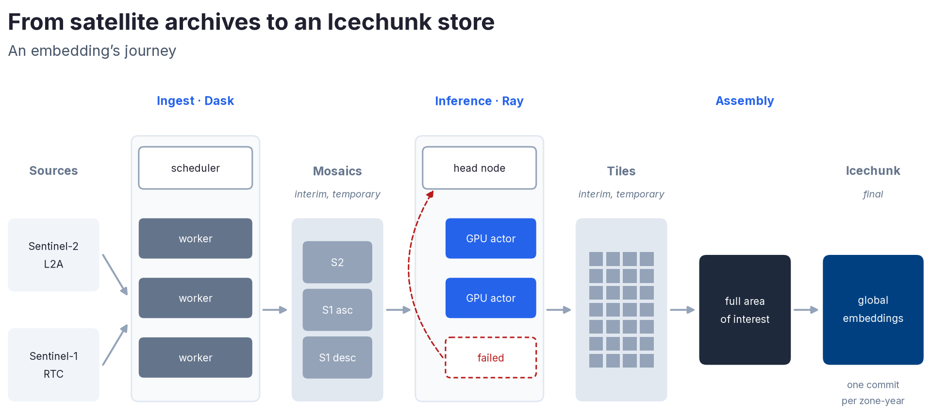
We built this system for internal projects first and were quite pleased with how it performed. Inevitably, the global campaign — processing the entire Sentinel-1 and Sentinel-2 archive — surfaced problems that only appear at scale. Until then we had only run the pipeline on instance counts in the low hundreds, enough for the mid-latitude agricultural areas we study at our parent company, Arbol. At larger scales, Dask’s schedulers became CPU-bound on large areas or with many hundreds of workers, falling behind and starving their workers of instructions and inputs. We invested significant effort in shrinking the scheduler’s task graph (more below) to take pressure off its CPU.

By happy contrast, once we had a well-functioning, work-stealing pool for inference, the Ray head node took ever-larger fleets in its stride. Had we been given two to five times as many GPU instances, we could probably have finished two to five times faster — something we hope to demonstrate the next time we generate these embeddings. This was our first time using Ray, and once past the initial learning curve we were very impressed with its stability and lack of fuss.

Performance optimizations

Ingest

Dask builds its entire task graph inside a single-threaded process, the scheduler, which hands tasks out to workers. Past a certain graph size, our fleet outran the overtaxed scheduler, and hundreds of machines sat idle waiting on that one saturated core.

The number of tasks in a graph is spatial chunks × dates × bands × operations, and each task costs the scheduler about 1.5 KB of memory. The bands were non-negotiable, so we shrank everything else: larger initial storage chunks, windows cropped to land and narrowed per date, one date per graph instead of a whole year, and the cloud and region masks fused into a single operation. Over a region 1,500 km by 1,000 km, a year’s work fell from 15.2 million tasks (22.8 GB) to just 38,000 (57 MB).

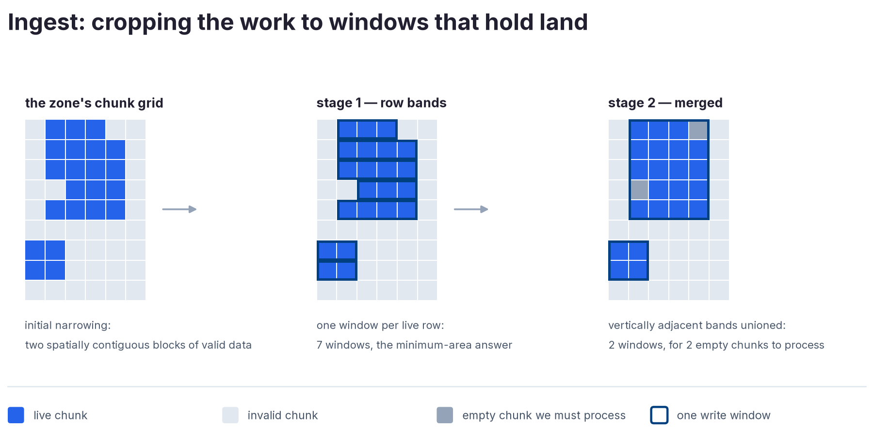
Many jobs contain areas we want to leave out: open ocean for global jobs, irrelevant geography for custom ones, and so on. By applying a mask of invalid 0.1 x 0.1 degrees tiles, and working only in chunk-aligned windows inside that mask, we cut the work (tiles) in our global campaign by 77%. Merging neighboring windows into single tasks trims the per-window overhead further.

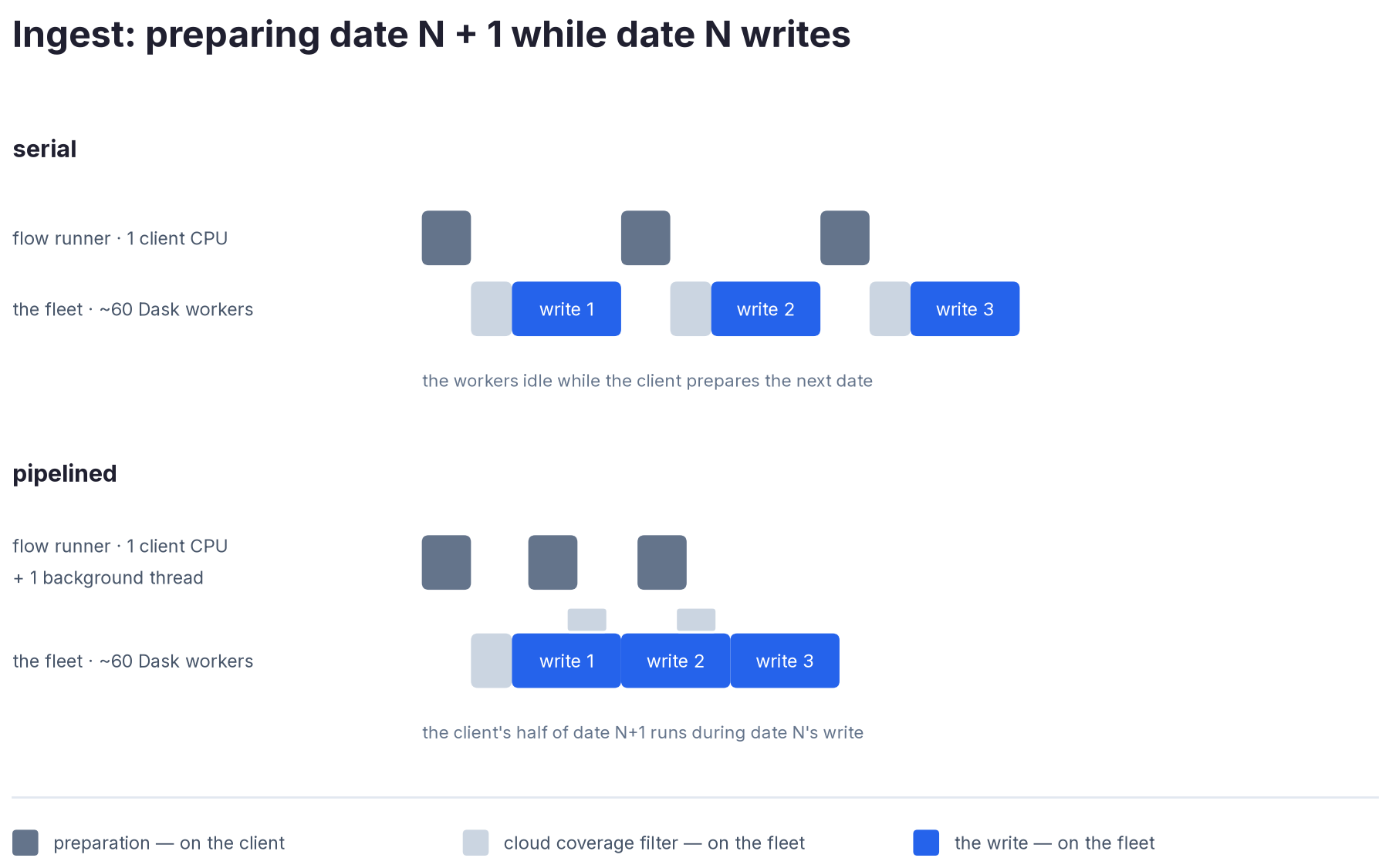
Preparing each date — building the load graph, running the cloud coverage filters, narrowing the footprint — reprojecting to our destination CRS — happens partly on the scheduler and partly on the workers. By doing the scheduler’s share while the workers are still busy, we hide its preparation time behind their writes. The cloud coverage filtering runs on those same workers, though, so preparing the filtering ahead of time only helps when they have CPU capacity to spare.

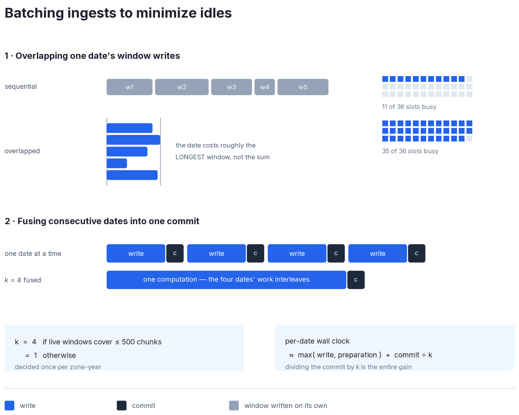
Each date’s pixels are written as several non-overlapping windows spread across many workers. Sent one window at a time, most of those workers sit idle. We cut write time dramatically by fusing into a single commit (a) all of a date’s windows and (b) several dates’ writes. The first runs sequential work in parallel; the second spreads the per-commit overhead across many writes. Together, these changes speed up satellite ingestion 2.5 to 4 times over a naive baseline.

Inference

Our goal in optimizing inference was to shave seconds off every tile, above all by eliminating wasted GPU idle time. This was the single most impactful work in the project: after implementing the changes we describe below, GPU utilization rose from about 50% to about 90% per run, idle time per tile fell from roughly a minute to a few seconds, each GPU processed 2 to 2.8 times as many pixels, and our overall project costs fell by over 40%.

We found efficiencies in several places in the model inference code itself. Vectorizing lookups and array gathers cut the time spent preparing each batch before it reaches the GPU. On the GPU itself, we consistently kept computation in BF16, fused the recurrent layer to reduce kernel launches, and set batch sizes large enough to keep the GPU fully occupied during matrix multiplication without stalling.

After these changes to the model code, we squeezed out further gains by re-engineering the inference process around it. Once a model’s batch size is well tuned, the forward pass typically becomes limited by memory bandwidth – how fast data gets moved onto and off of the GPU tensor cores – rather than compute. Specifically, fleet telemetry from the naive sequential version showed the GPUs’ multiprocessors active most of the time, while the tensor cores — the parts of a GPU that do the actual matrix math — were engaged less than half of that time. In effect, they spent much of each cycle waiting for data.

Keeping the GPU much, much busier was therefore our most important task: to fix that, we broke the work into smaller pieces and fed them to the GPU as one continuous, uninterrupted stream. But how? A 2048-pixel tile, one year deep, is too large for our GPU instances to hold at once: far larger than our preferred AWS g6e.xlarge’s 46 GB of VRAM, and larger than the worker’s RAM budget too.

The answer is to stream each tile through the tensor cores in strips and load/write in parallel with processing. The GPU can only work on what has arrived, so its idle time falls into three windows: loading, saving, and the gaps mid-forward-pass while it waits for the next sub-batch. After the first tile, the only remaining pause is the copy from host memory to the card before each sub-batch. The pipeline runs on a single CUDA stream, so a copy and a forward pass can never fully overlap.

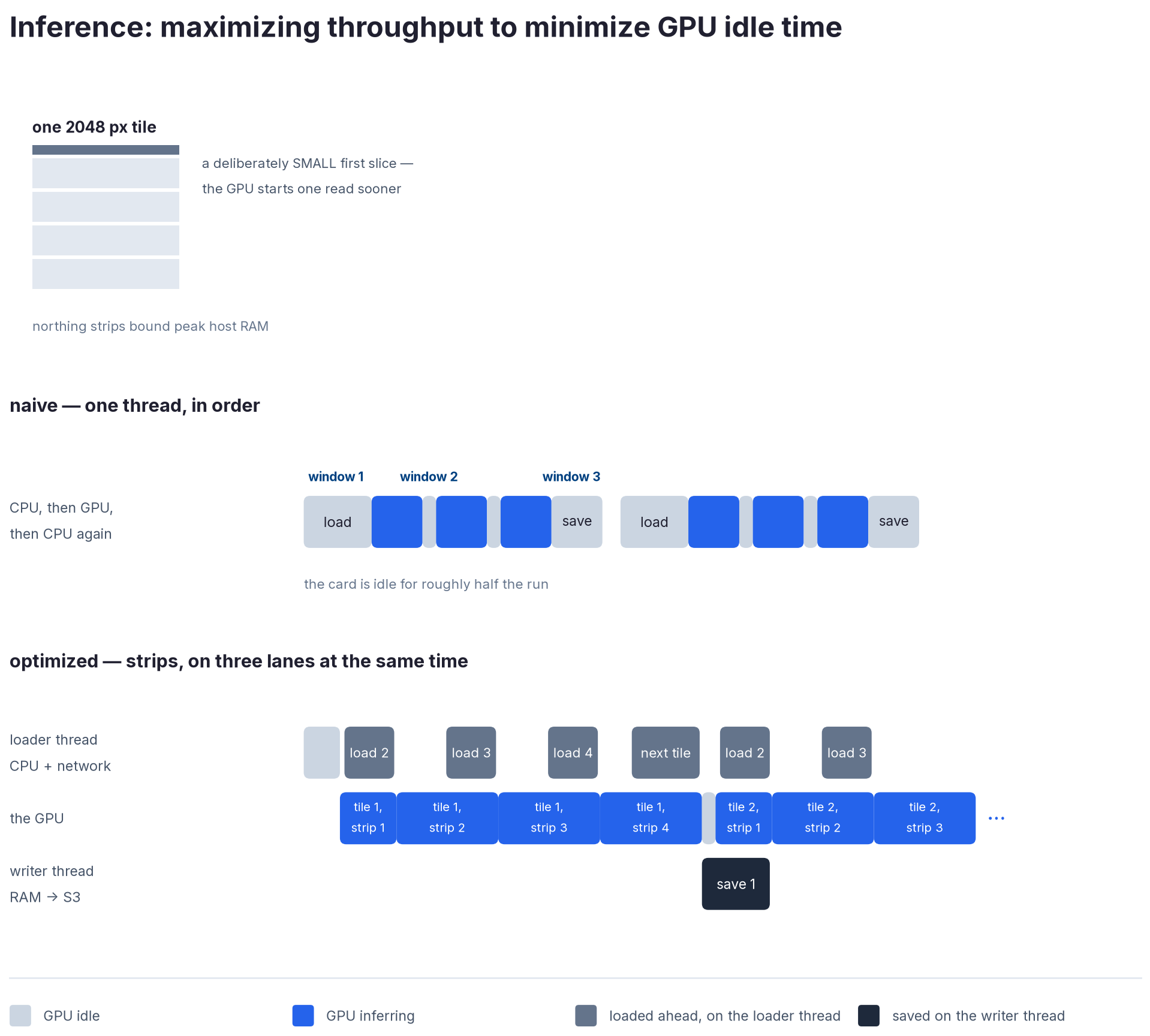
Inside the GPU tensor core, splitting each tile into east-west strips bounds peak host memory and lets us hide the loading of one strip behind the processing of the one before it. Reading the first strip of the next tile while the last strip of the current one is being processed means the GPU starts on the next tile about 6 seconds after finishing the last, rather than 24 to 36. Whether a tile is split at all, and whether prefetching is worth it, is decided per tile from its valid-pixel count. A tile dense with valid observations has enough work to hide its loads; a sparse tile with few valid pixels has memory to spare, so it turns prefetching off and reads fewer, larger areas. 

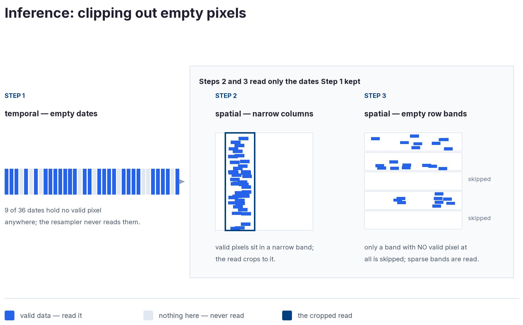
We found further gains by clipping invalid (cloudy or masked) pixels out of each strip, so workers only spend time moving and inferring pixels we will actually use. Sentinel-2’s SCL cloud mask tells us which dates and which areas of a tile hold no usable data and can be safely skipped. Which optimizations apply depends on the tile. A dense inland tile crops nothing and prunes little, so its speedup comes from striping and prefetching. A cloudy or coastal sliver is the opposite: its valid-pixel count is so low that it fits in memory as a single strip, and reading only its valid pixels is the big win. Most tiles fall somewhere in between.

Data assembly

Assembling the staged, inferred tiles was the least technically complicated part of our stack, but we quickly learned that moving terabytes or petabytes of data gets unwieldy when done the wrong way. We first tried distributing the work with a small Dask cluster, but that made the scheduler’s task graph overhead scale with both our chunk size and the size of the area covered, even when most of it was empty. The second of those bit us hard once we went global: for sparse areas, the task graph was wildly out of proportion to the actual work. 

After some head-scratching, we dropped the Dask middleman and used the Zarr library directly, moving blocks of data into the final store with plain array assignment in forked worker processes. Crucially, because our inference tiles and our final shards are both 2048 × 2048 pixels, each holds exactly 64 of our 256 × 256 inner chunks, so no rechunking is needed. This is faster and uses far less memory, which let us consolidate assembly onto a single beefy 32-vCPU machine.

Data store

In Cambridge’s original implementation, data was processed and stored as 5 km × 5 km tiles, each a directory of NumPy arrays. NumPy is a poor fit for a massive cloud store. It stores each array as a single uncompressed, unchunked run of values, so a partial read is only efficient along one axis, and cloud array tools cannot read it lazily. It also records an array’s type and shape but nothing geospatial: georeferencing, dates and band metadata live in sidecar files, and a tile’s location is encoded only in its directory name.

We settled on Icechunk, the open-source storage engine maintained by the excellent team at Earthmover. Icechunk sits underneath Zarr, the N-dimensional array format, and adds transactions, git-style commits and other core features of a traditional database. That gave us far more confidence that our operations were safe to repeat: if a write failed or was interrupted, we could — and repeatedly did — simply restart, where a plain Zarr store would have been left corrupted. So we ended up using (and interrupting) Icechunk stores for both our final data product and the interim satellite mosaics.

Even pushed to petabyte scale, with up to 10 simultaneous writes and commits, Icechunk largely just worked. Commits and writes flowed smoothly, interruptions caused no issues, and read performance (about 325 ms for one pixel and 2.8 s for a 4096 × 4096 block, in-region on AWS) held up at our final 1.6 petabytes. We came away genuinely impressed.

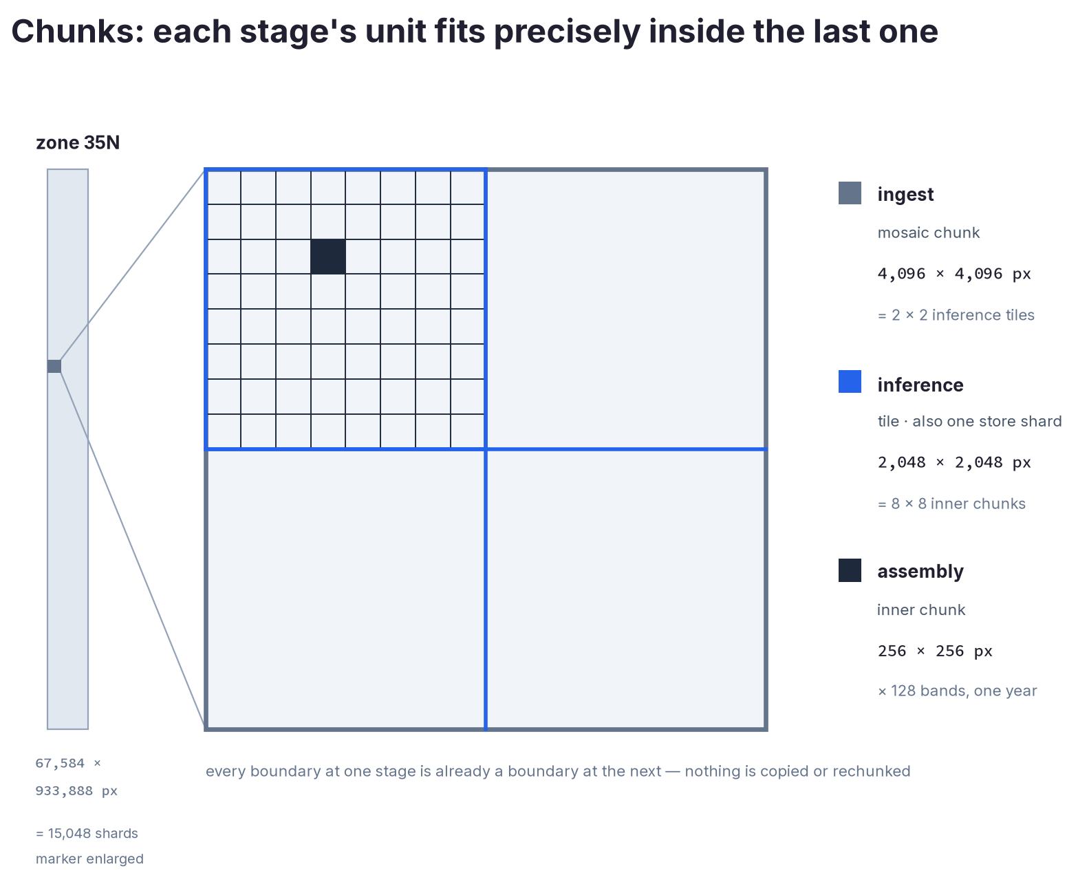
Beyond Icechunk itself, we tuned our storage parameters for writes and reads through a structured series of stress tests on a realistically sized and structured Icechunk store. Those tests settled us on balanced chunk and shard sizes that divide evenly into one another across stages: 4096 × 4096 pixels for ingest (mosaics), 2048 × 2048 for inference (staging), and 256 × 256 for inner chunks. Keeping those sizes evenly divisible was fundamental, because it spared us expensive copy and rechunk operations every time one stage’s output became the next stage’s input.

A note on our process

This being 2026, we should be upfront that we leaned heavily on AI to speed up development. Letting Claude drive meant we could iterate through our own ideas fast, build rigorous stress tests faithful to our production stack, write extensive documentation, and exhaustively profile the inefficient parts of our stack — usually a major pain in distributed environments. Traditional engineers at heart, we weren’t exactly thrilled to lean on AI so much and write so little by hand, but there was no other way for a tiny team to build a stack we’re genuinely proud of.

It also showed the value of building directly on a validated, peer-reviewed model from the excellent team at Cambridge. Because our results could be verified, we could use AI far more aggressively: we cross-validated our independent implementation against theirs, and whenever we got the same results on downstream tasks, we could proceed with full confidence, even after substantially rewiring the model’s inference internals. It’s a perfect demonstration of the power of open source, open data, open validation benchmarks and open publishing.

Conclusion

The best thing about all of the above? It's yours too, if you want it. Evan and I have developed our code in the open at every step, in dClimate's tessera-embeddings GitHub repository, and validated it with our friends at Cambridge over Zulip.

We invite users, collaborators and critics to take a look, and, if you’re feeling adventurous, to generate your own embeddings. Go ahead and play with it! Sub-annual embeddings for small areas like cities can be computed locally in minutes on a good workstation. 

If you’re so inspired, run it yourself at scale, or improve it with a pull request to the repository. Join the dClimate Discord to share what you're building with TESSERA and see what else we have in store. If you have questions about TESSERA itself (or just want to watch the sausage being made), join the TESSERA Zulip chat. We hope this is just the beginning.